Quickstart : A journey throught the Iris dataset

Introduction

The Iris flower dataset is a multivariate dataset introduced by the British statistician and biologist Ronald Fisher in his 1936 paper "The use of multiple measurements in taxonomic problems" as an example of linear discriminant analysis. It consists of 50 samples from each of three species of Iris (Iris setosa, Iris virginica and Iris versicolor). Four features were measured from each sample: the length and the width of the sepals and petals, in centimeters. The Iris dataset is widely used in machine learning as a benchmark dataset for statistical classification algorithms. It is free and publicly avaible at the UCI Machine Repository.

The following tutorial allows to illustrate main Chalk'it features througth this dataset. Expected result is provided in the following project:

• iris-tutorial.xprjson

1. Create a projet

Run Chalk'it in the command line:

chalk-it

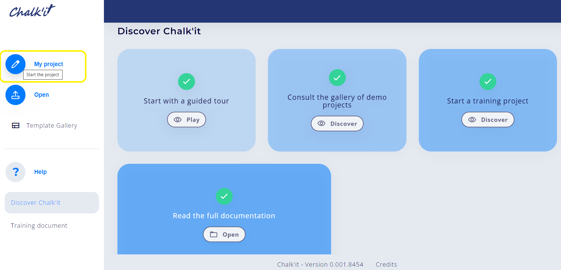
Then, click My Project button to reach project editor on the Discover Chalk'it menu.

Name the new projet iris-tutorial by filling the title form, then save it using the Save button.

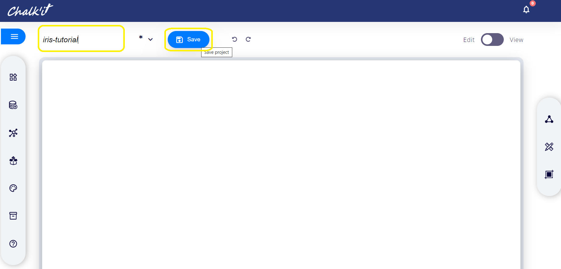
An iris-tutorial.xprjson is then created in your current directory (directory where the chalk-it command was run).

2. Load required Python Pyodide librairies

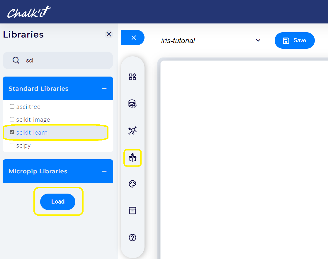
Using the Project librairies main tab, load the following required librairies: pandas, scikit-learn (from the Standard Librairies tabset) and plotly (from the Micropip Librairies tabset). Use the search bar to ease the process.

3. Load dataset data

Create a datanode named dataset to load the Iris dataset from Scikit-learn by following the next instructions:

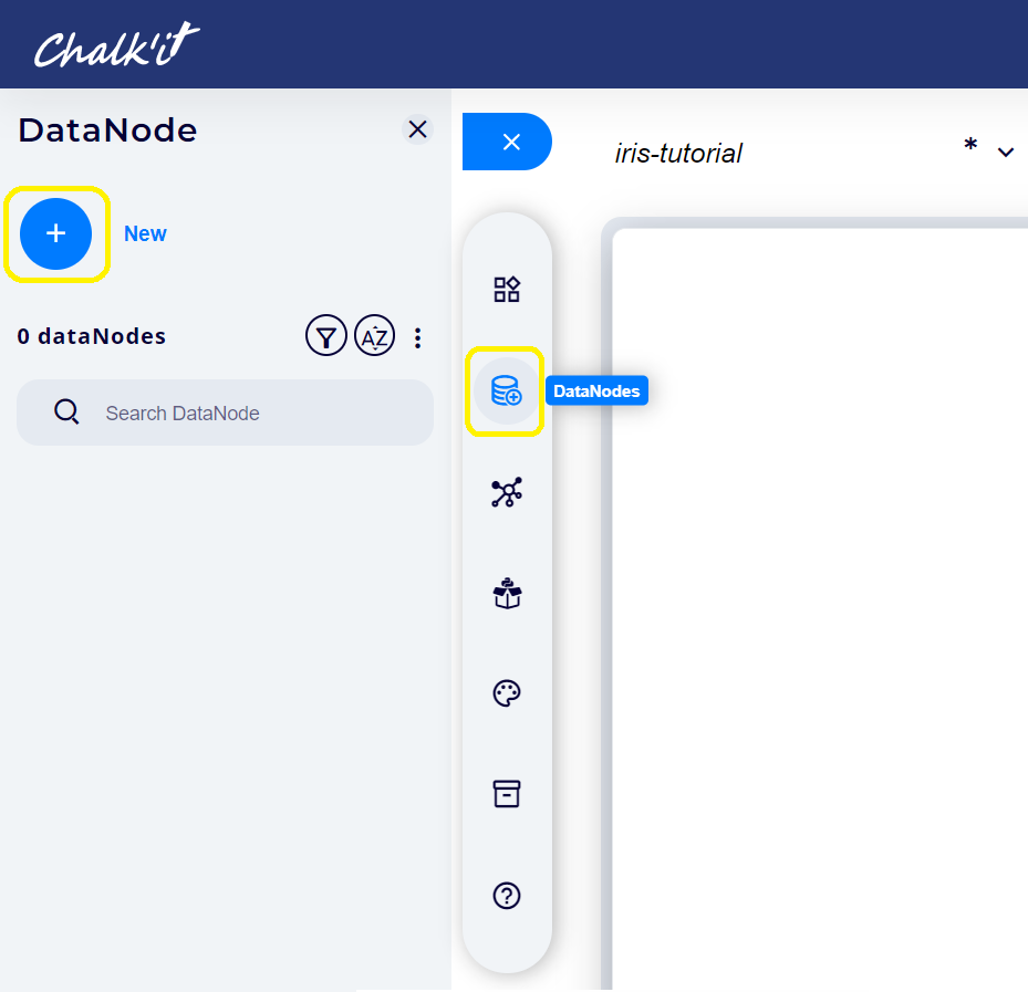
• Click on Datanodes main tab, then on New button:

• Select Script (Pyodide) from the list of datanode types:

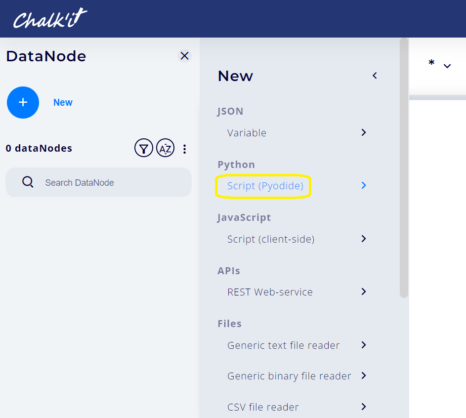
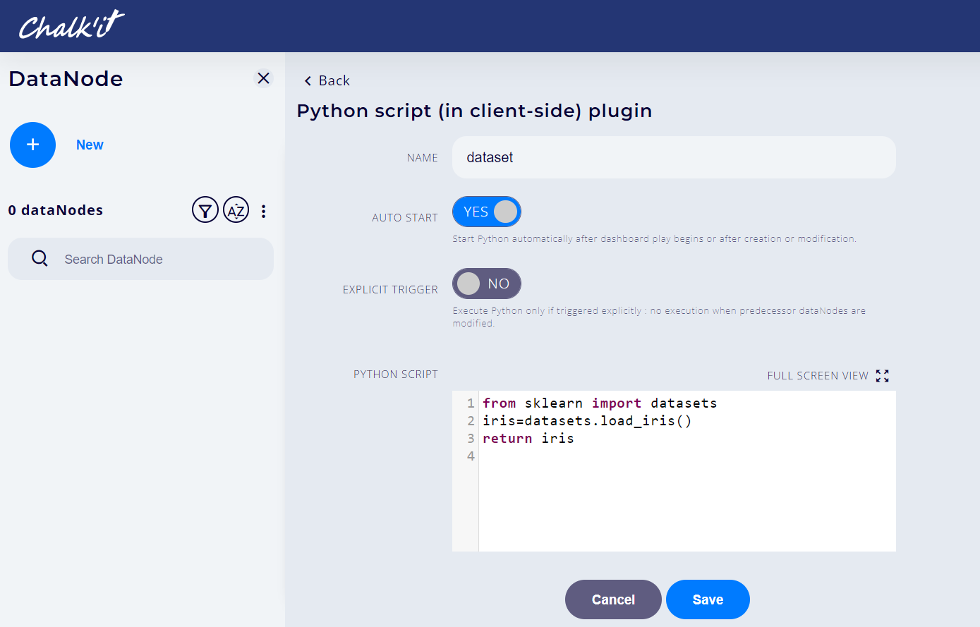
• Enter dataset in the NAME field and copy the following code into the PYTHON SCRIPT field:

from sklearn import datasets
iris=datasets.load_iris()
return iris

This step is illustrated below:

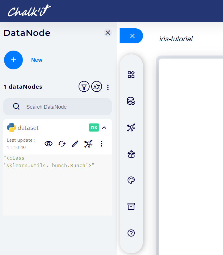
• Finally, click on Save button for validation.

Datanode execution status and result are now available and can be previewed in the dataset window as follows:

4. Visualize the dataset

Visualize the dataset in 4 steps:

Step1: prepare the data

• To load the dataset in a Pandas dataframe, follow the procedure described in paragraph 2. to create a new Script (Pyodide) datanode. The main differences are:

• Enter datasetDataframe in NAME field,

• Copy the following code in PYTHON SCRIPT field.

import pandas as pd

iris=dataNodes["dataset"]

df = pd.DataFrame(data=iris.data, columns=iris.feature_names)
df["target"] = iris.target
target_names = {0: "Setosa", 1: "Versicolour", 2: "Virginica" }
df['target'] = df['target'].map(target_names)

return df

The expression dataNodes["dataset"] indicates Chalk'it to read the last execution output of the dataset datanode. It also establishes a data and execution flow dependency between dataset and datasetDataframe.

• To visualize the dataset using Plotly Python librairy, create a new Script (Pyodide) datanode, name it plot, then copy the following code in PYTHON SCRIPT field.

import plotly.express as px

df = dataNodes["datasetDataframe"]
fig = px.scatter(df, x="sepal width (cm)", y="sepal length (cm)", color="target", size='petal length (cm)', hover_data=['petal width (cm)'])

return fig

Step2: create the dashboard

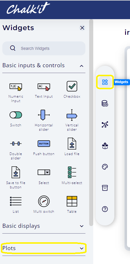
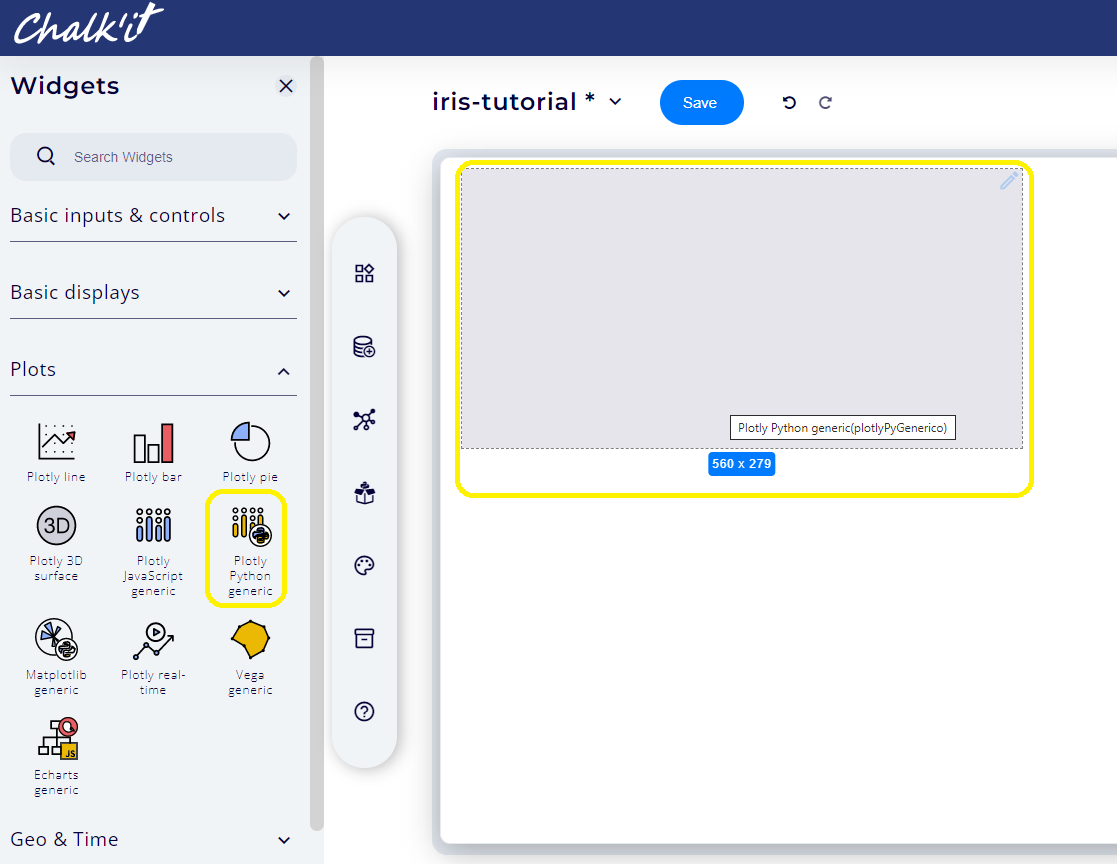
• To browse the widgets libraries, click on Widgets main tab, then open the Plots category as shown below:

• To add a Plotly Python widget to the dashboard editor, click on the corresponding icon or just perform a drag and drop.

Step3: connect dataNode to widget

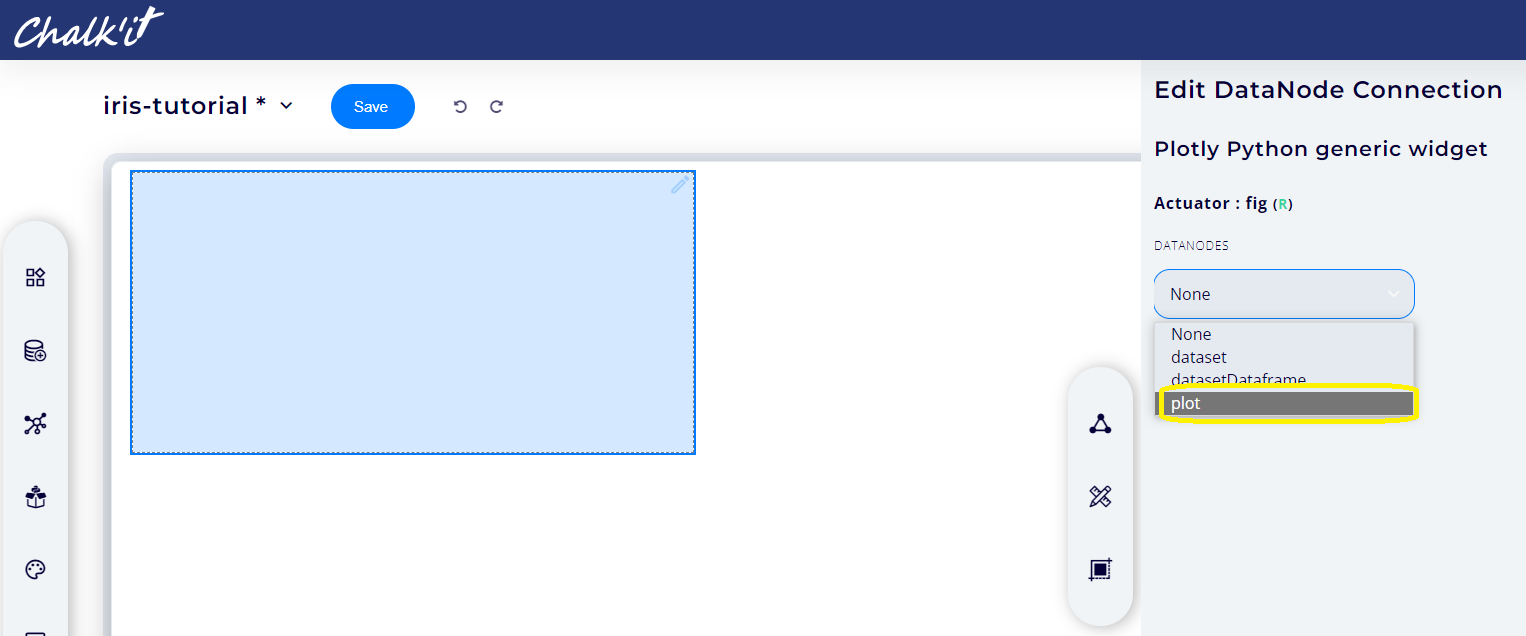
• Click on the pencil icon on the top-right corner of the widget to display the widget menu. Select then Connect widget as shown below:

• A panel will then be displayed on the right-side of the screen. From the connection dropdown, select the datanode plot, as it will provide the figure object needed for the widget. Click Save to validate the choice.

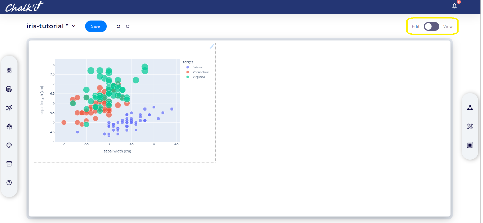
Step4: Preview the dashboard

• A static preview of the figure is then provided. The widget can be moved or resized as needed. The *View* mode can be selected to start interactive visualization.

5. Interactive predictor with classifier training

The goal is now to use the previously trained classifier to predict Iris species based on petal and sepal width and length.

Classifier training

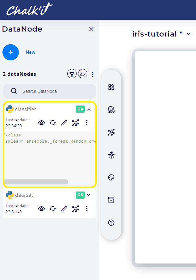
Following the steps already described in paragraph 2., create a Script (Pyodide) datanode named classifier and use the following python script as shown in the picture below.

from sklearn.ensemble import RandomForestClassifier
clf=RandomForestClassifier()
clf.fit(dataNodes["dataset"].data,dataNodes["dataset"].target)
return clf

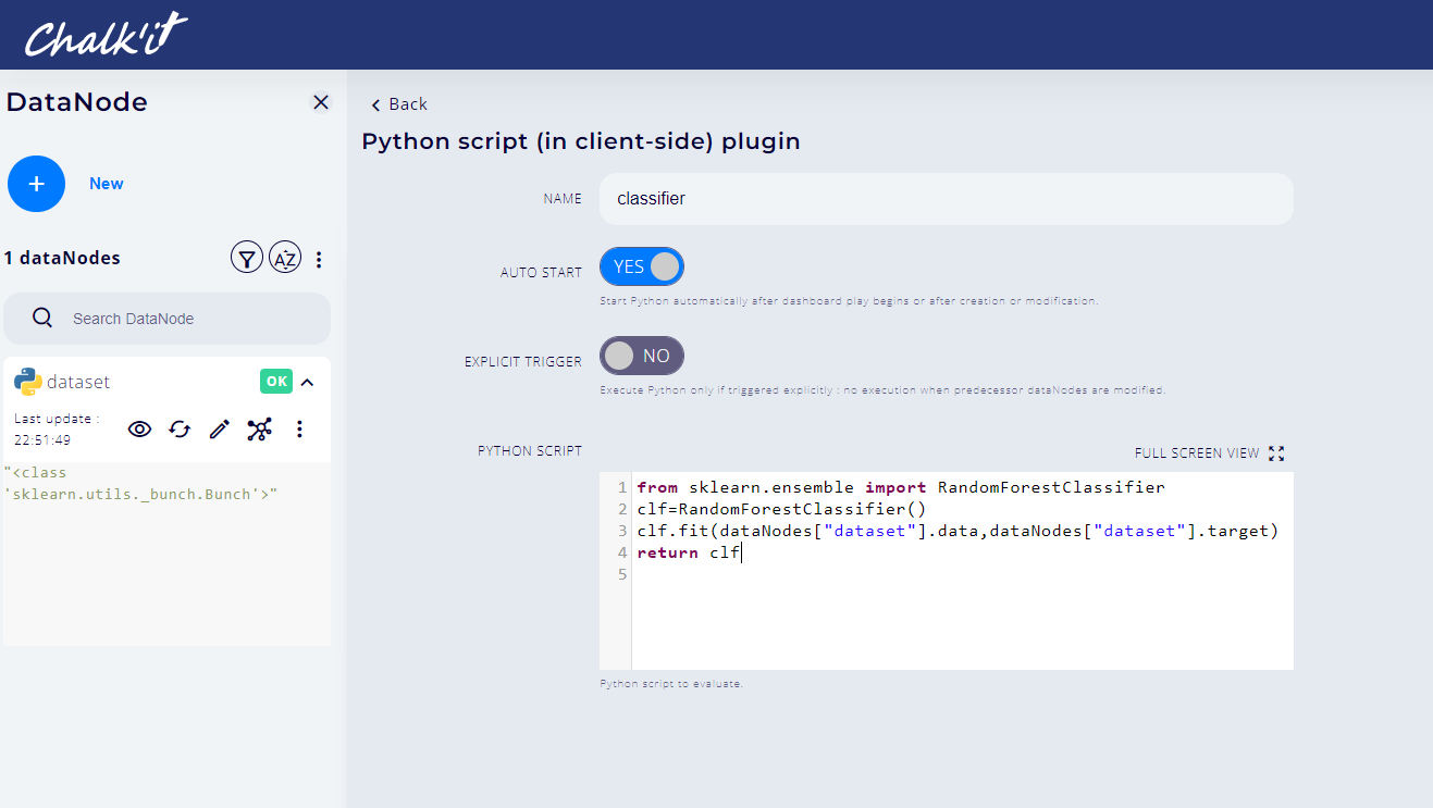
The result should look like:

Interactive predictor

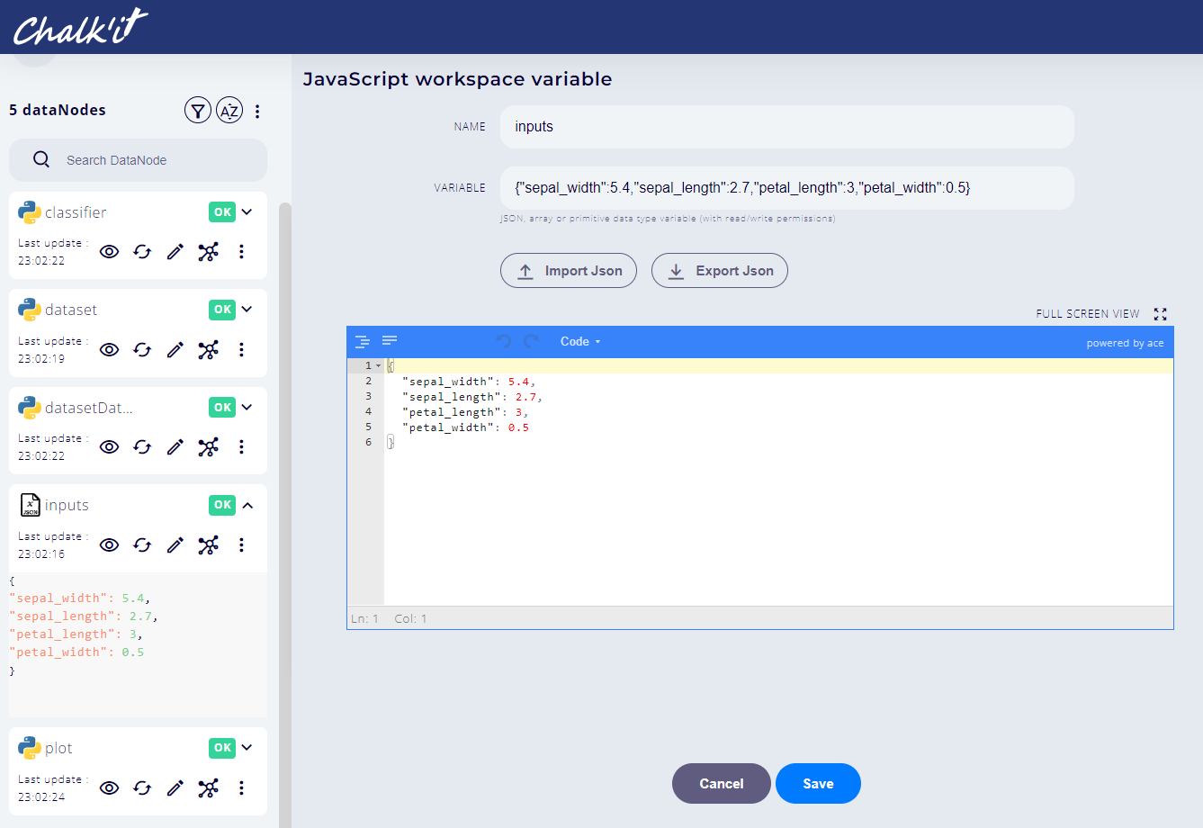
• Create a JSON Variable datanode named inputs using JavaScript workspace variable type. Use the following JSON definition:

{"sepal_width":5.4,"sepal_length":2.7,"petal_length":3,"petal_width":0.5}

The result should be as follow:

• Add four horizontal sliders to pilot the values of "sepalwidth","sepal_length", "petal_length" and "petal_width". First click the _Widgets main tab, then basic inputs & controls.

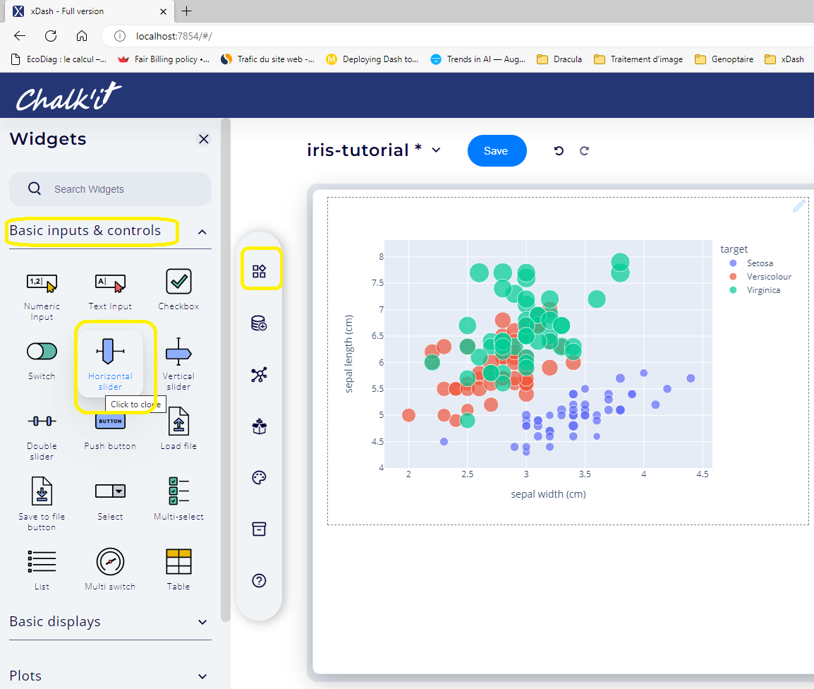
• Connect each slider to its corresponding feature as shown below:

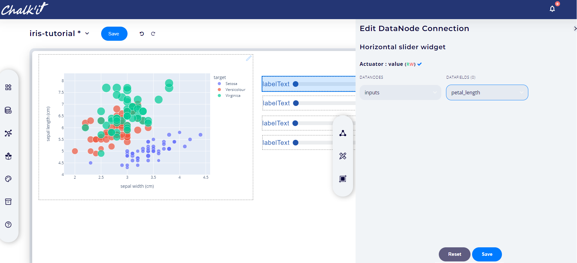
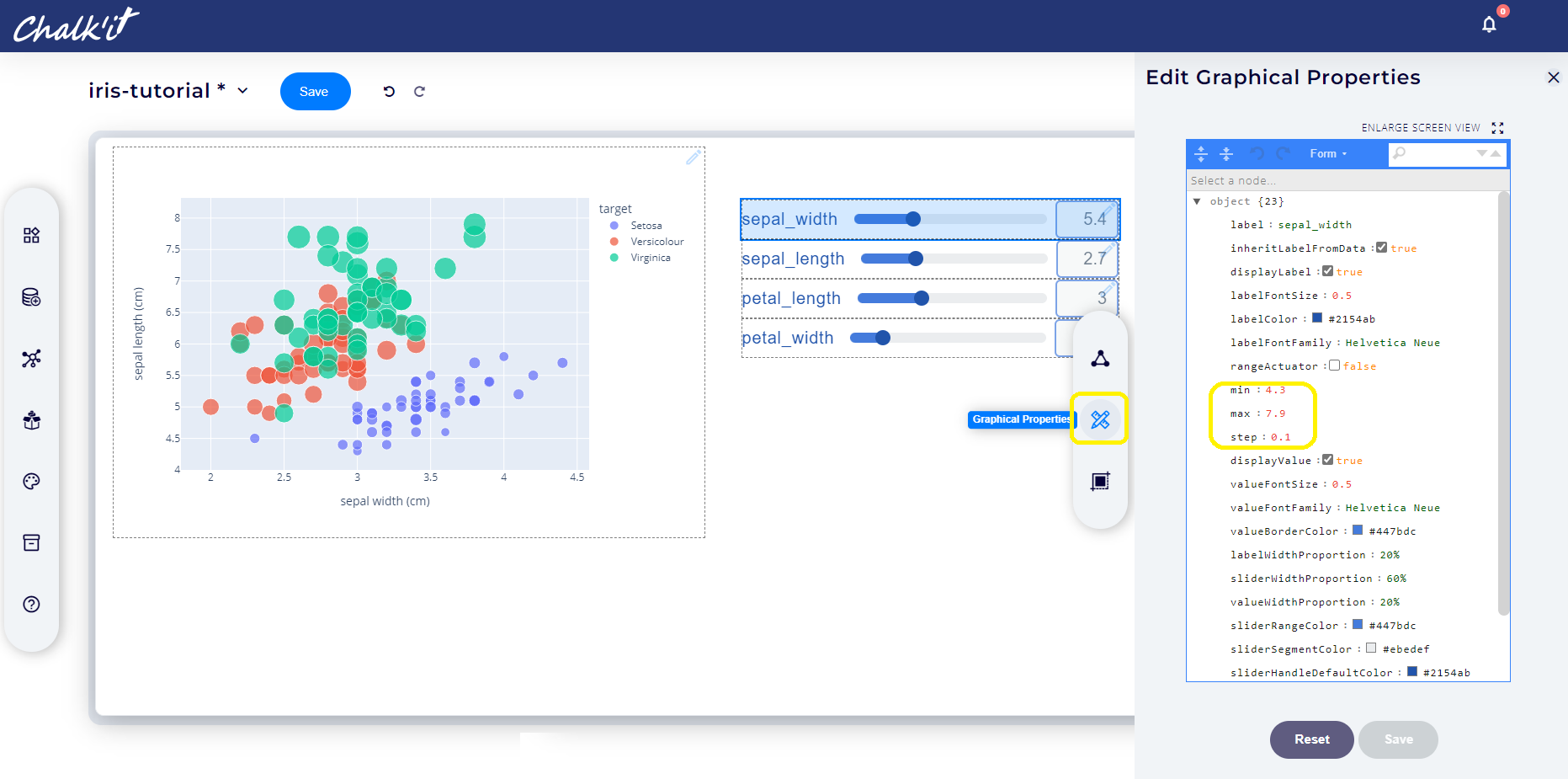
• Configure sliders properties with a sliding step of 0.1 and min/max values as stated in the following table:

Feature	min	max
sepal_width	4.3	7.9
sepal_length	2.0	4.4
petal_width	0.1	2.5
petal_length	1.0	6.9

For this purpose, select the Graphical properties tab of each widget as illustrated below:

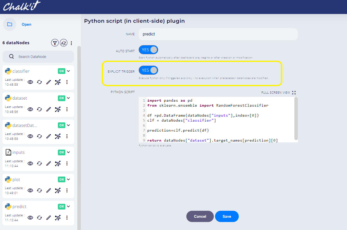
• Add a Script (Pyodide) datanode named predict with the following code:

import pandas as pd
from sklearn.ensemble import RandomForestClassifier

df =pd.DataFrame(dataNodes["inputs"],index=[0])
clf = dataNodes["classifier"]

prediction=clf.predict(df)

return dataNodes["dataset"].target_names[prediction][0]

• Go back to the Widgets main tab, open the Basic Displays tabset, and then add a KPI value widget

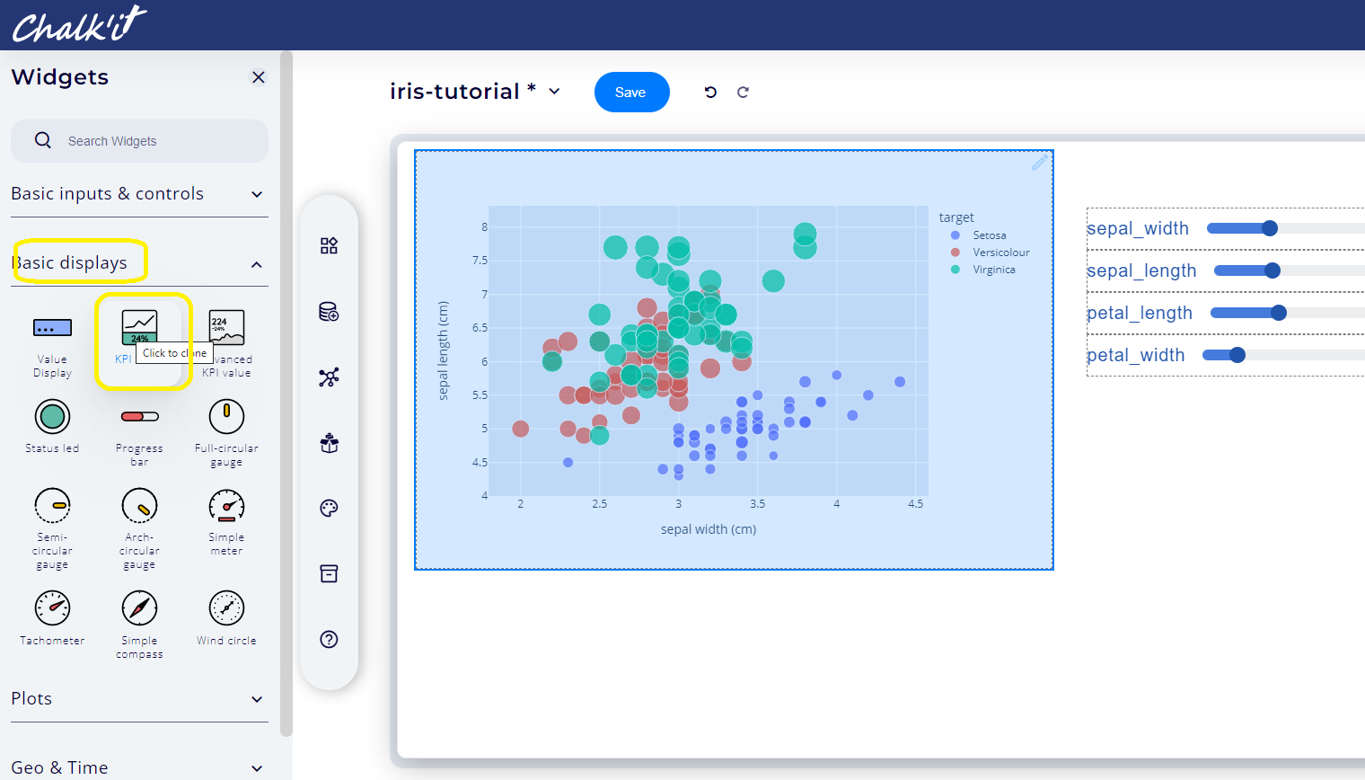
• Connect this widget to the predict datanode.

• Switch to *View* mode. Use the sliders to change Iris features and view prediction result accordingly:

Note that computation will be triggered every time a slider is changed.

Explicit trigger

Sometimes a different behaviour is needed, a form-like behaviour where the predictor execution is triggered only when a button is clicked.

This behaviour can be achieved through the following steps :

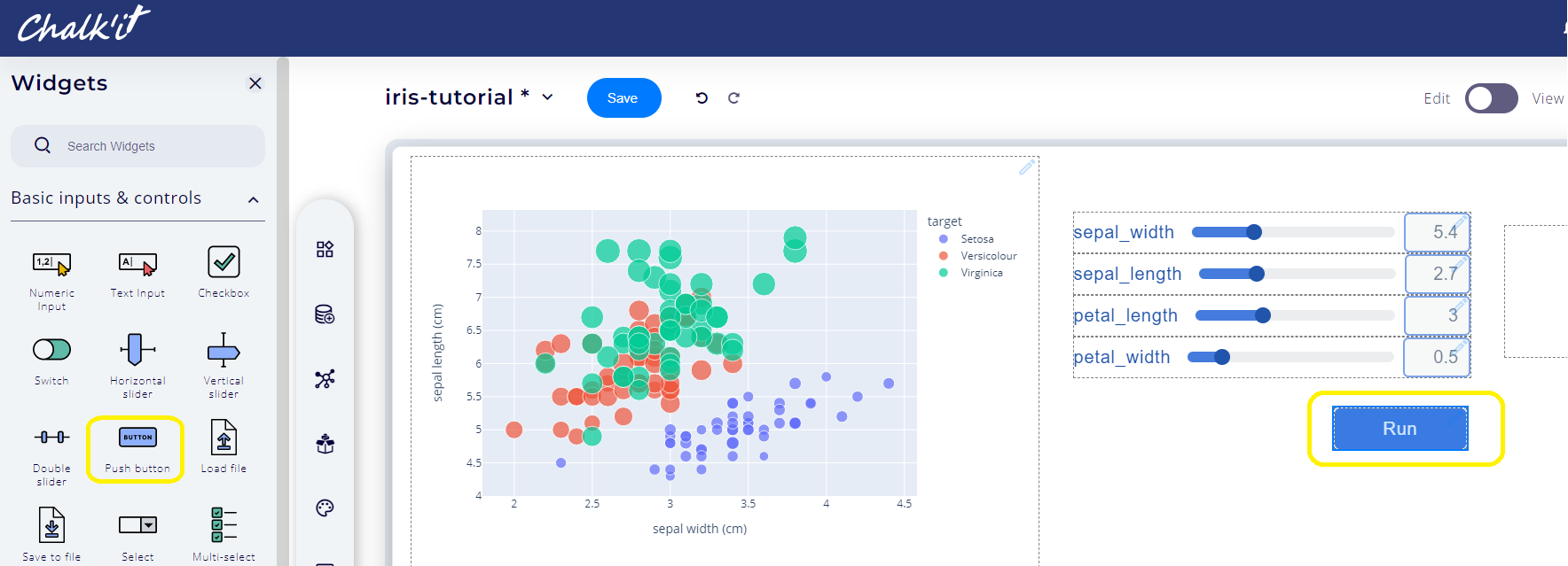
• Switch to *Edit* mode. Add a button widget, connect it to the predict datanode, and name it Run.

• Open the datanode predict, switch the EXPLICIT TRIGGER parameter to YES.

• Switch back to *View* mode to test the new behaviour.

• This project, when finished, can be previewed or exported to a standalone HTML page or your app can be deployed and shared using a public or a private link.